Hydronics Workshop | John Siegenthaler
What’s it capable of? (part 1)
Why accurate performance measurements are essential when evaluating an existing hydronic system for a heat pump.
Contractors can verify current system capacity and supply-temperature requirements before committing to an air-to-water heat pump retrofit.
When asked about adding an air-to-water heat pump to an existing heating system, you need a way to evaluate how the existing distribution system and heat emitters can work with that heat pump.
If the existing system was designed around high-water temperatures, such as 180 ºF, you might dismiss the use of a heat pump because it cannot produce the high temperature water at which the system was originally designed to operate. However, there may be more to the “evolution” of that system than what you initially think.
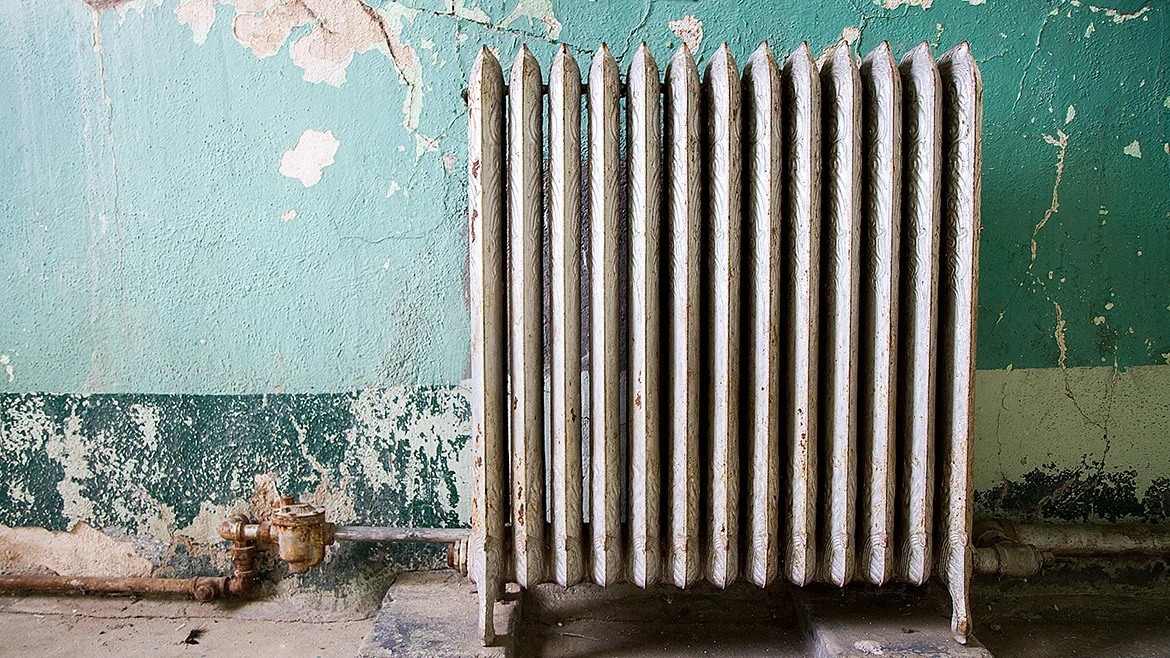
The building might have been weatherized since the original system was installed, and its design heating load is now significantly lower. Lower heat loss means that lower water temperatures can be used in the same distribution system. Perhaps a second-hand cast-iron radiator or new fan-coil has been added to the original distribution system, which would also lower the required supply water temperature. There are many possibilities for how the original hydronic heating circuits, or the building they heat, have been modified over the years.
How can you evaluate the thermal performance of the distribution system in its current condition, accounting for any modifications to it or the building it serves?
One approach is to make theoretical hydraulic and thermal “models” of each circuit. To do this, and keep the results accurate, you’ll need to measure the lengths of all the piping, count all the fittings and valves, look up pump curves for the circulators, and even check what fluid is in the system (e.g., water or an antifreeze solution). You’ll also need to measure the finned-tubing length in all the baseboards and look up heat output data for any other heat emitters in the circuits. Once you have all this data, you’ll need to make several calculations, some of which can be challenging. This is all possible, but it’s a LOT of work, and the results are only as accurate as the data and formulas used for those calculations.
Measure rather than model
An alternative approach is to measure the thermal performance of the circuit as it operates. To do this, you’ll need instruments that can accurately measure the temperature drop around the circuit as it dissipates heat. You’ll also need to measure the flow rate through the circuit.
A dual-channel thermocouple meter, such as the one shown in Figure 1 is ideal for simultaneously measuring two temperatures, one at the beginning of the circuit and the other at the end. These meters can also display the difference between those temperatures.
FIGURE 1
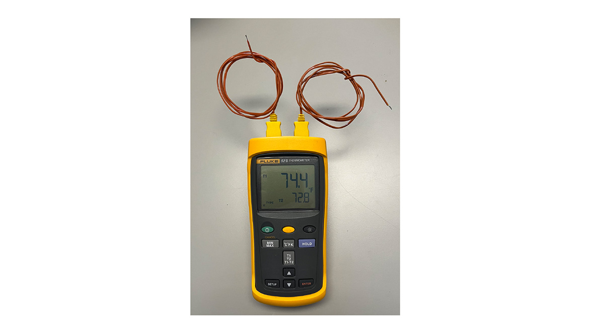
Image courtesy of John Siegenthaler
This meter comes with two thermocouples, which are very small “junctions” between two types of wire at the end of the lead. Because thermocouples are very small, they’re easy to mount and fast responding. They can be temporarily held to the surface of a copper tube using electrical tape. A short sleeve of elastomeric foam insulation should then be used to cover the thermocouple to minimize any influence of surrounding air on the temperature reading.
Measuring the flow rate through a circuit has always been more of a challenge compared to measuring temperatures. Very few circuits are equipped with permanently installed flow meters. Devices such as balancing valves, when paired with instruments such as digital manometers, can provide flow rate estimates, but with accuracies only in the range of +/-10 to 15%. The cost of installing those valves along with purchasing a digital manometer to convert the differential pressure across them to a flow rate usually precludes their use in residential systems, especially as devices that would need to be retrofitted. Imaging telling a prospective customer that you need to install several hundred dollars worth of flow metering hardware just to assess how their system performs, with no assurance that the results would bode well for using a heat pump… Next in line please…
Clamp rather than cut
One of the most convenient devices for accurately measuring flow rates through pipes is an ultrasonic flow meter. These meters work by recording the “flight time” of a high frequency (ultrasonic) wave as it travels through the fluid, first in the direction of flow, and then in the opposite direction. The meter converts the difference in these flight times to the volumetric flow rate through the pipe. They do this while being mounted on the outside surface of the pipe.
When first introduced, ultrasonic flow meters cost thousands of dollars, but they are now available, for pipe sizes up to 1.25 inch, in the price range of $400-600. Figure 2 shows an example of one such meter from KEYENCE.
FIGURE 2
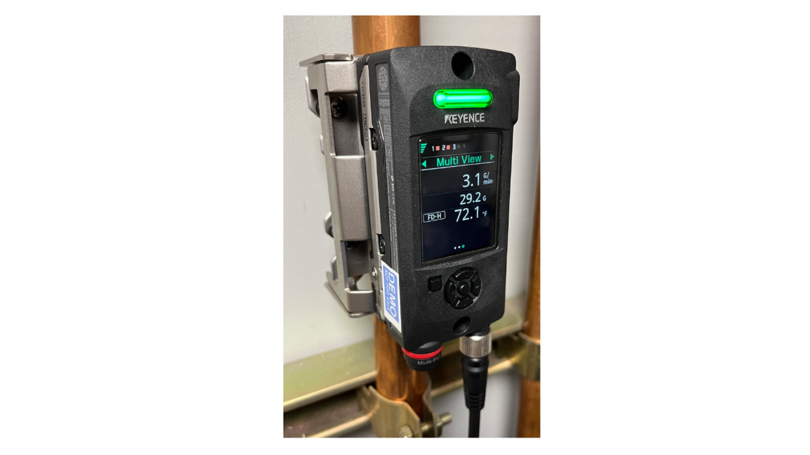
Image courtesy of John Siegenthaler
This meter comes with a mounting frame that clamps to the outside of the pipe. With a small battery-powered screwdriver, that frame can be secured or removed in about 30 seconds, so it’s easy to move the meter from one circuit to another. The electronic portion of the meter clips onto this frame and is powered by a small “black box” 12 VDC power supply.
The KEYENCE meters can work on a variety of piping materials, and with a wide range of fluids. They can also resolve flow rate to the nearest 0.1 gpm with a listed accuracy of +/- 3% of the reading.
Holding it steady
One of the “nuances” of measuring the thermal performance of a hydronic circuit is taking the measurements while the circuit is operating under steady state conditions. The means that the temperature change (e.g., ∆T), and flow rate are both holding steady for at least several minutes. This is necessary to ensure that the thermal mass of the circuit is not absorbing or releasing heat. When operating at steady state, the heat input to the circuit equals the heat output from the circuit. When a circuit operates under transient rather than steady state conditions, the temperature change and flow rate measurements don’t provide an accurate indication of what the circuit is capable of.
Circuits that have relatively low thermal mass - such as shorter circuits of small diameter tubing serving fin-tube baseboard or a fan-coil - can reach steady state in a few minutes if the heat input rate to the circuit is steady. Circuits through cast-iron baseboard or radiant floor panels may take hours to reach a true steady state condition.
Systems with “on/off” heat sources seldom operate at steady state conditions. When the heat source is on, the thermal mass of the circuit is absorbing heat. When the heat source is off, the thermal mass of the circuit is releasing heat.
One way to circumvent this issue is to use a heat source that can be controlled to yield a very steady rate of heat input to the circuit. An electric resistance heating element with minimal thermal mass is one such source. Figure 3 shows one possibility.
FIGURE 3
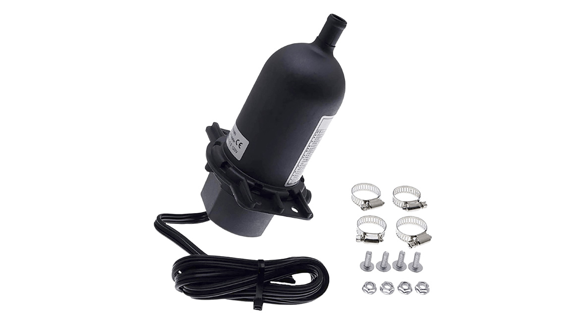
Image courtesy of John Siegenthaler
This is 1500 watt electric “block heater.” It’s designed for warming the coolant in vehicle engines prior to starting them under extremely cold conditions. It’s a simple and inexpensive device, just a shell with inlet and outlet ports and an internal heating element.
One nice thing about an electric resistance heat source is that it’s easy to control the rate at which it turns electricity into heat and adds it to the system fluid. The power input to the block heater is easily controlled by a solid state “dimmer,” such as the one shown in figure 4.
FIGURE 4
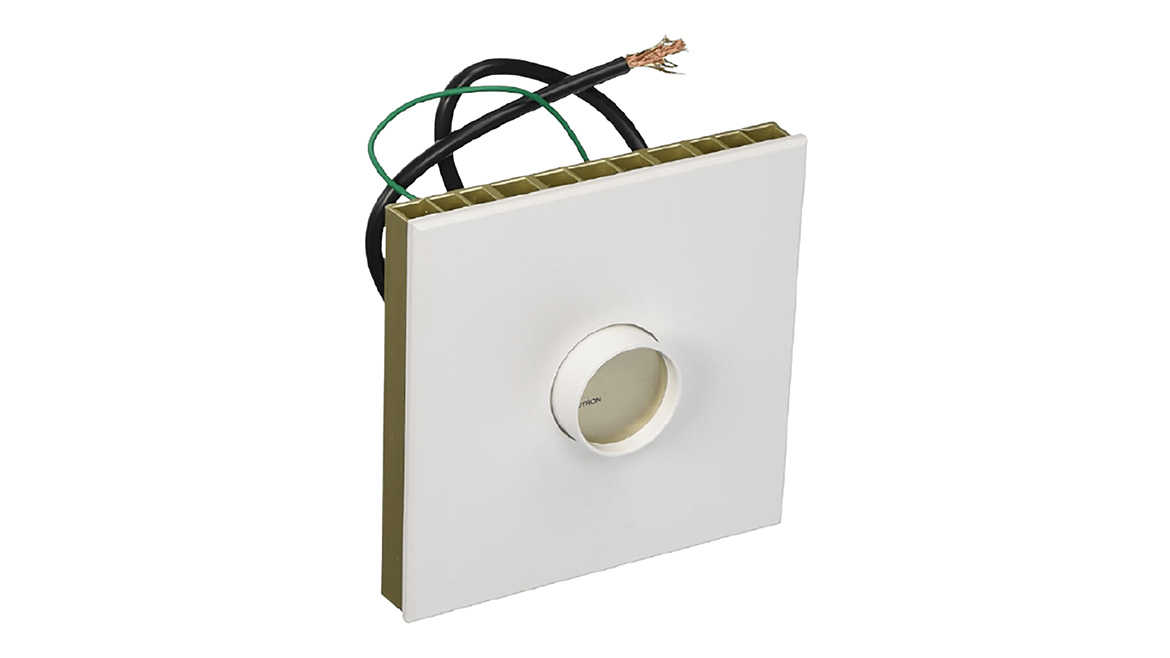
Image courtesy of John Siegenthaler
The solid-state dimmer needs to have a power rating at least as high as that of the device it controls. A solid-state dimmer with a rating of 2000 watts is capable of fully controlling the power input to the 1500-watt block heater. These devices are about 99% efficient, implying that 1% of the power they receive is converted to heat. At a full 2000-watt input, that’s a heat dissipation of 20 watts. Hence, the heat sink fins on the device.
Another nice thing about an electric resistance heat source is the ability to measure the rate of energy transfer. It could be done by simultaneously measuring the voltage across the heating element, and the amperage flowing through the element. Multiply the voltage by the amperage to get the wattage, as shown in formula 1.
Formula 1:
Where:
P = power supplied to the element (watts)
i = current flowing through the element (amps)
v= voltage supplied to the element (volts)
An even easier way to measure the power to the element is by using a small watt meter such as the KILL A WATT meter shown in figure 5.
FIGURE 5
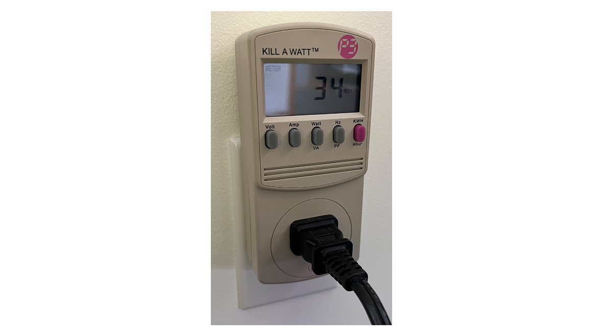
Image courtesy of John Siegenthaler
The KILL A WATT meter shown is rated for resistance heating loads up to 1875 watts. It, along with the solid-state dimmer and block heater can be connected as show in figure 6.
FIGURE 6
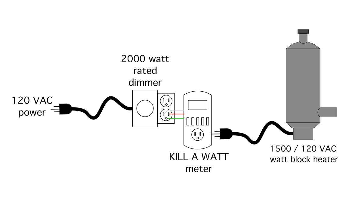
Image courtesy of John Siegenthaler
The apparatus
The easiest way to get the block heater along with a variable speed circulator, and other hardware details into the circuit for testing is to close the isolation valves on the circulator flanges, remove the existing circulator, and insert the test apparatus as shown in figure 7.
FIGURE 7
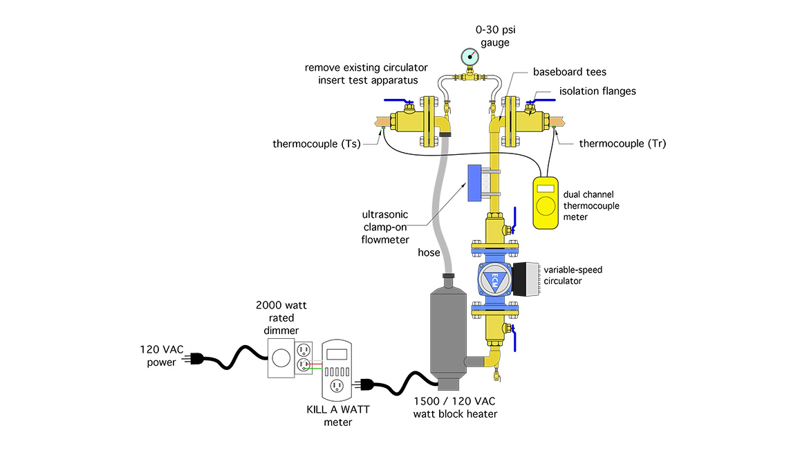
Image courtesy of John Siegenthaler
This apparatus becomes the temporary heat source and flow source for the circuit. The variable speed ECM circulator can be adjusted over a wide range of flow. Heat input to the circuit can be adjust from 0 to 1500 watts (0 - 5,120 Btu/hr). The temperature drop of the circuit is measured using the dual channel thermocouple meter, and flow is measured with the ultrasonic flow meter.
Measuring the flow rate through a circuit has always been more of a challenge compared to measuring temperatures. Very few circuits are equipped with permanently installed flow meters.
The baseboard tees connecting to the circulator flanges provide two 1/8” FPT ports which can be connected using two ball cocks and fuel line to a single pressure gauge. By opening one ball cock at a time the pressure on the supply side and return side can be measured. The difference between these pressures can be converted to head. By measuring the pressure difference at several flow rates, and converting those pressure differences to head, it’s possible to create a circuit head loss curve. That curve can then be used to evaluate the flow rate that any specific circulator could create in the circuit.
More to follow
I suspect many readers have a pretty good idea of how to use the testing apparatus shown in figure 7. Just dial up some heat, measure the flow rate and temperature drop, and make a simple calculation. Well, that is the general idea, but there are several details that need attention to ensure that the data is accurate and that it truly representative of what the circuit is capable of. We’ll get into those in next month’s column.
Looking for a reprint of this article?
From high-res PDFs to custom plaques, order your copy today!