Hydronics Workshop | John Siegenthaler
What’s it capable of? (part 2)
Measuring net heat output and head loss in existing hydronic circuits.

Using field measurements to eliminate guesswork in hydronic design.
Last month, we began a discussion on testing the thermal and hydraulic performance of existing hydronic heating circuits. That testing involved the apparatus shown in figure 1.
FIGURE 1
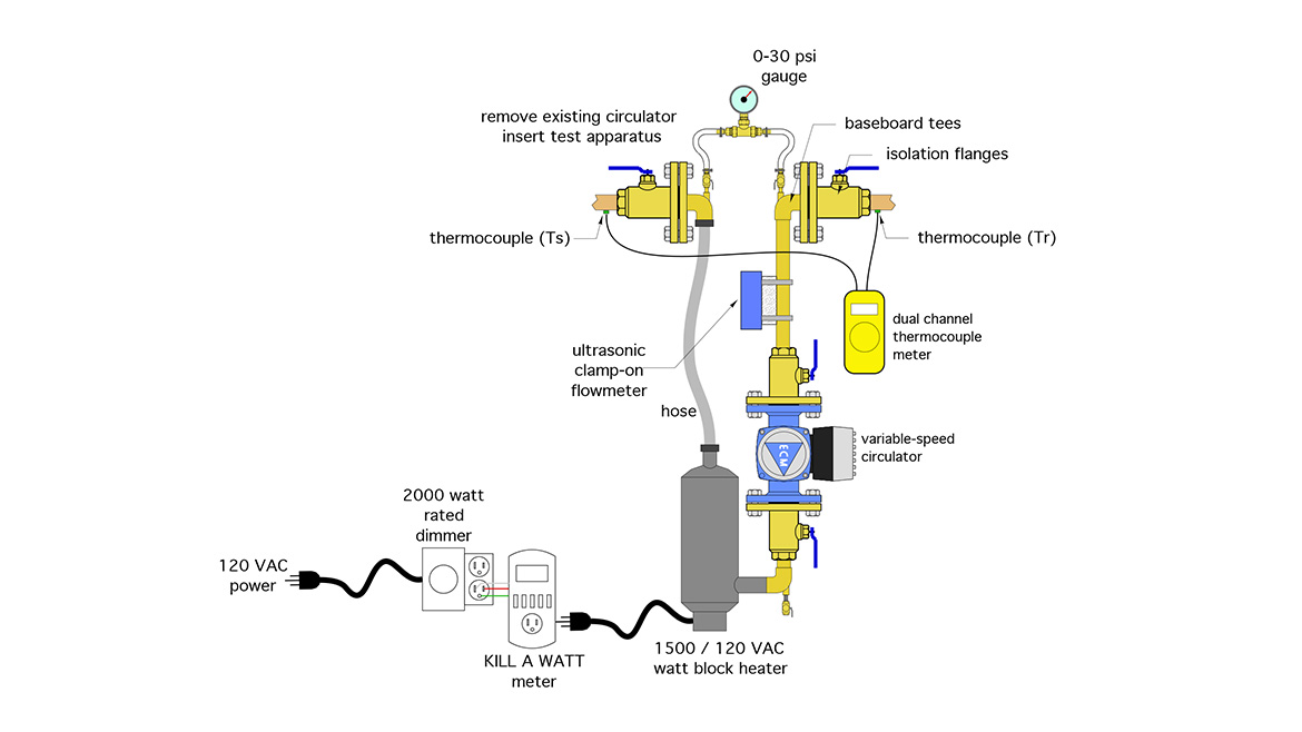
Drawing courtesy of John Siegenthaler
This apparatus becomes the temporary heat source and flow source for the circuit, and mounts between a set of existing circulator flanges in the circuit. The variable speed ECM circulator can be adjusted to create a wide range of flow rates. The solid state dimmer allows heat input to the circuit through the block heater to be adjusted and measured from zero to 1500 watts (0 - 5,120 Btu/hr). The temperature drop of the circuit is measured using the dual channel thermocouple meter, and flow is measured with the ultrasonic flow meter.
Heat source vs. heat loss
In many hydronic systems, the circuit being tested passes through the boiler. Under normal operation, that boiler adds heat to the circuit; but when the block heater in the test apparatus is the heat source, and the boiler is off, the latter is dissipating heat from the circuit. This heat dissipation would not be present in normal operation of the circuit, and it needs to be accounted for when measuring the true “net” heating output ability of the circuit. That net heat output can be calculated using formula 1.
Formula 1:

Courtesy of John Siegenthaler
Where:
q = rate of heat dissipated from circuit (Btu/hr)
8.01 = a constant required by the units used
D = density of the fluid at the average temperature of the circuit (lb/ft3)
c = specific heat of the fluid at the average temperature of the circuit (Btu/lb/ºF)
f = measured flow rate through circuit (gpm)
∆Tcircuit = measured temperature drop of circuit (ºF)
∆Tboiler = measured temperature drop across the inactive boiler (ºF)
The term ∆Tboiler would be the measured temperature drop across the boiler when the testing is taking place at steady state conditions. The dual channel thermocouple meter can be used to accurately measure this temperature drop. Having another set of thermocouples installed between boiler’s inlet and outlet allows the meter to be quickly moved to read the ∆T across the boiler.
If the boiler is connected to the distribution system using closely spaced tees, or through a hydraulic separator, any heat dissipation from the boiler during the test should be insignificant. Still, it’s a good idea to close off any valve that can temporarily stop flow through a boiler connected to the distribution system in this manner.
Ready when steady
It’s important that the circuit is operating at steady state conditions when the temperature and flow measurements are taken.
It’s not important that the supply water temperature to the circuit during the test is the same as would be provided by the boiler under normal operation.
Keeping the supply temperature in the range of 20-25 ºF above surrounding air temperature typically allows the circuit to reach steady state faster than what time would be required to get the circuit up to about 170 or 180 ºF. It may not even be possible for the 1500-watt electric heater to get the circuit to these higher temperatures.
Step 1: The first step in testing a circuit takes place before the test apparatus is installed. Turn on all zone circulators, or open all zone valves, but keep the boiler off. This creates maximum flow and maximum head loss through the common piping. It also creates minimum flow through each zone circuit. This condition provides a “conservative” flow condition under which to evaluate each circuit.
Step 2: With all zones operating, use the ultrasonic flow meter to measure the flow rate in each circuit and record it.
Step 3: Install the test apparatus shown in figure 1 in one circuit, and adjust the circulator’s speed to establish a flow rate approximately equal to that measured in step 2.
Step 4: Turn on the solid state dimmer and KILL A WATT meter, and adjust the power input to the block heater. Try to get the circuit to settle to a steady state when the supply temperature is 20-25 ºF above the surrounding air temperature.
Step 5: Once steady state conditions are established, measure and record the temperature drop around the circuit using the dual channel thermocouple meter. While the circuit is still operating at the same conditions, measure and record the temperature drop across the inactive boiler.
Step 6: Use the graphs in figure 2 to get values for the density and specific heat of the fluid being circulated. Use the average fluid temperature in the circuit when looking up these values on the graph.
FIGURE 2
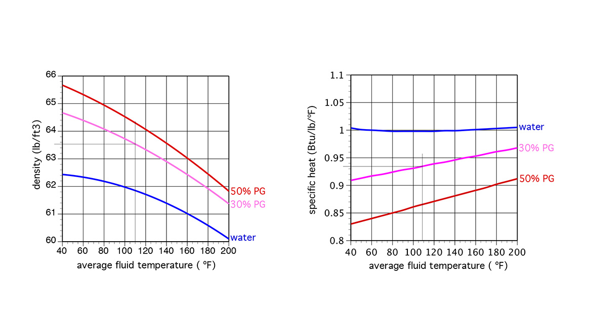
Drawing courtesy of John Siegenthaler
Step 7: Use formula 1 to calculate the net heat output of the circuit, record it along with the supply water temperature to the circuit.
If there’s more than one circuit in the system, reinstall the original circulator in the circuit just tested, move the test apparatus to the next circuit, and repeat the testing procedure until all circuits have been tested.
Extrapolation
After testing the circuit(s) and using formula 1, you should have values for net heat output, along with the corresponding supply water temperature. Those numbers are probably not in the normal operating conditions of the circuit; no worries. This is where a fundamental relationship that forms the basis of outdoor reset control can be applied. Specifically: The heat output of any hydronic circuit is approximately proportional to the difference between the supply water temperature and the surrounding air temperature. This relationship can be represented by formula 2.
Formula 2:
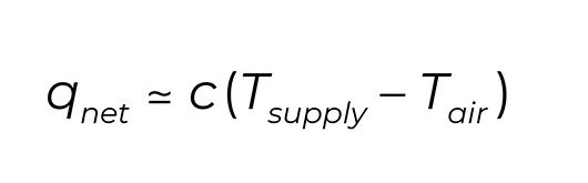
Courtesy of John Siegenthaler
Where:
q = circuit heat output rate (Btu/hr)
c = a number to be determined
Tsupply = temperature of fluid supplied to circuit (ºF)
Tair = temperature of air surrounding the circuit (ºF)
The “squiggly” equal sign means approximately equal to.
The value of (c) in formula 2 can be determined based on the net heat output of the circuit, along with the corresponding supply water temperature and air temperature recorded from the testing.
For example: Consider a circuit that - at steady state conditions - had the following measured operating conditions:
Tsupply = 100 ºF
Tair - 75 ºF
calculated net heat output using measured data and formula 1 = 5,400 Btu/hr
The value of c for this circuit is calculated as follows:
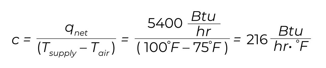
Courtesy of John Siegenthaler
To find the heat output of the circuit at other supply water temperatures or other surrounding air temperatures, just put those temperatures along with the value of (c) into formula 2.
For example: What is the approximate output of the circuit with the c value of 216 Btu/hr/ºF when supplied with water at 125ºF and with a surrounding air temperature of 68 ºF? Putting these values into formula 2 and calculating yields:
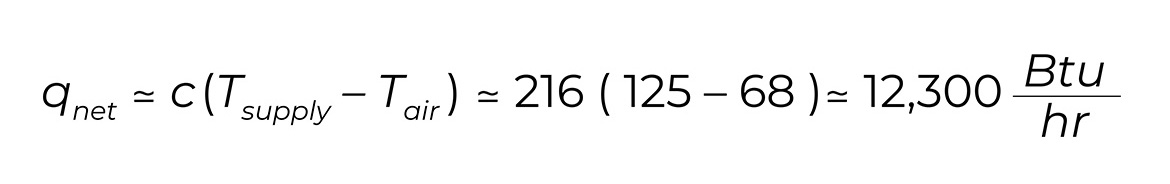
Courtesy of John Siegenthaler
Now that the value of (c) for the circuit is established, you can use formula 2, along with the circuit test data, to get a reasonable estimate for the circuit’s heat output rate over any reasonable range of supply water temperature. However, it’s best to limit the range of air temperatures used in formula 2 to no more than 5 ºF above or below the air temperature at which the circuit was tested. This is especially true for circuits that have piping in spaces with different air temperatures. There are ways (albeit complicated) to separate out all the heat output from piping and heat emitters on a circuit that passes through spaces with different air temperatures, but that’s well beyond the testing described above and - trust me - it’s best left to computers.
Curves that cross
Every hydronic circuit, no matter how properly or poorly designed, has a unique relationship between the flow rate passing through it and the resulting head loss. That relationship is called the circuit head loss curve.
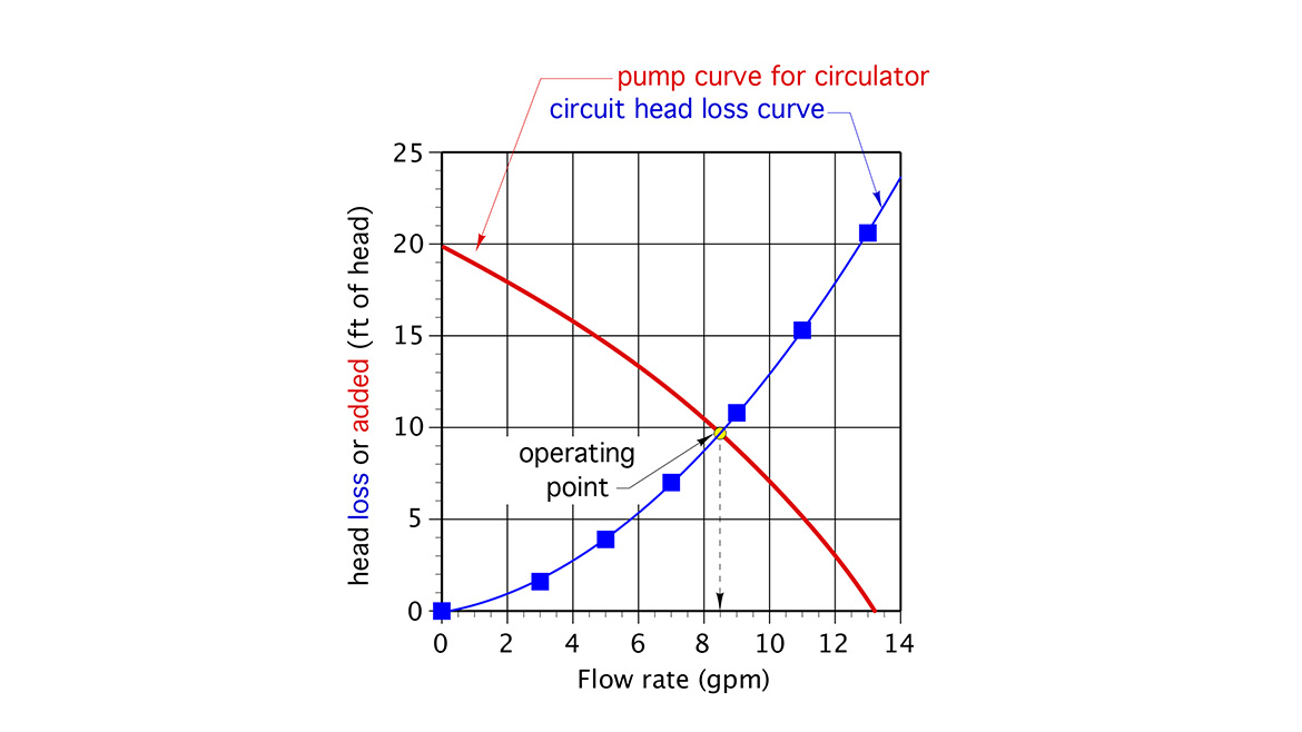
The circuit head loss curve can be plotted on the same graph as the pump curve of a “candidate” circulator being considered for the circuit. The point at which the circuit head loss curve crosses the circulator’s pump curve is called the operating point. A line drawn straight down from this point shows the flow rate that would exist in the circuit when powered by that circulator.
Figure 3 shows a typical circuit head loss curve, a pump curve and the corresponding operating point.
FIGURE 3
Drawing courtesy of John Siegenthaler
The test apparatus can be used to collect data that can be plotted to create the circuit head loss curve. The data points, when plotted, are represented by the blue squares in figure 3.
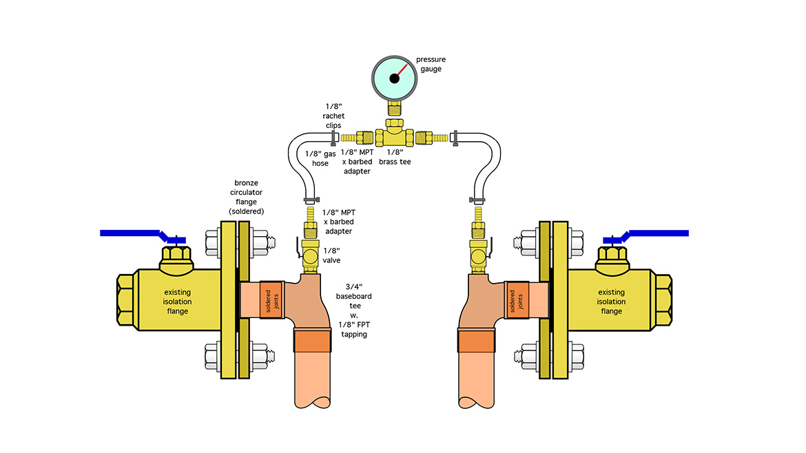
Figure 4 shows a detailed view of the hardware in the upper portion of the test apparatus.
FIGURE 4
Drawing courtesy of John Siegenthaler
The baseboard tees provide two 1/8” FPT connections into the circuit, one on the supply side of the test circulator and the other on the inlet side. These connections lead to two small ball valves and on through two short segments of fuel line that connect to a tee with a pressure gauge. The small fittings shown in figure 4 all exist, although perhaps not on the shelves at your local wholesaler. I’ve found that several online sources offer them.
The pressure gauge used needs to have a range that’s high enough to handle the static pressure in the system, and also show the difference between supply and return side pressures with the best accuracy. Since most residential and light commercial systems have static pressures in the range of 10-15 psi, a pressure gauge with a range of 0-30 psi is usually OK.
By opening one of the small ball valves at a time, it’s possible to get the pressure on the supply and return sides of the circuit. The difference between these pressure readings is the “∆P” at which the circuit is operating at the current test flow rate.
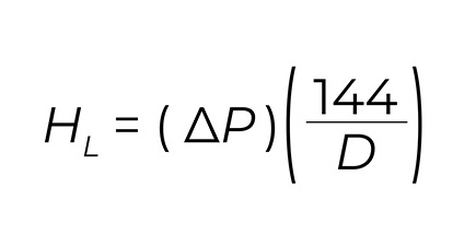
To create the circuit head loss curve, it’s necessary to convert the ∆P data to head loss using formula 3.
Formula 3:
Courtesy of John Siegenthaler
Where:
HL = head loss of the circuit (feet of head)
∆P = pressure drop of the circuit (psi)
D = density of the fluid in the circuit (lb/ft3) (read from figure 2)
144 = a constant based on the units used.
The test procedure is straight forward:
Step 1: Choose several flow rates that the circuit could operate at. For example, a circuit made of 3/4” copper tubing could operate with flow rates up to perhaps 10 gpm. Although 10 gpm in a 3/4” tube would create a flow velocity much higher than a suggested limit of 4 feet per second, it could exist if an oversized circulator was used. So, for a range of 0-10 gpm, the test flow rates could be 2, 4, 6, 8 and 10 gpm. They don’t have to be even or whole numbers, they just have to cover a reasonable range of flow rates that could exist in the circuit.
Step 2: Use the variable speed circulator and the ultrasonic flow meter on the test apparatus to establish each of these test flow rates in the circuit, one at a time.
Step 3: Measure the circuit’s supply side and return side pressure at each test flow rates. Subtract the return side pressure from the supply side pressure and write down the ∆P that occurred at each test flow rate.
In many hydronic systems, the circuit being tested passes through the boiler. Under normal operation, that boiler adds heat to the circuit; but when the block heater in the test apparatus is the heat source, and the boiler is off, the latter is dissipating heat from the circuit.
Step 4: Convert each ∆P to head loss using formula 3. Use figure 2, along with the average circuit temperature to get the density of the fluid.
Step 5: Use spreadsheet software to graph the test data for head loss versus flow rate. One point that isn’t measured but still should be included on the graph is 0 head loss at 0 flow rate. Use the spreadsheet’s curve fitting function to create a smooth curve connecting the dots. The result is the circuit’s head loss curve.
The data points can also be plotted on a graph that shows one or more pump curves for circulators being considered for the circuit.
A professional approach
The test apparatus described in this column and last month’s column should be thought of as a profession tool. It’s easy to build, and affordable. Its use allows the thermal and hydraulic performance of a hydronic circuit to be measured to an accuracy that’s sufficient for evaluating how the circuit would operate at different supply water temperatures or with a different circulator. It’s use replaces “guessing” with measuring, the latter being the approach a professional would choose.
Looking for a reprint of this article?
From high-res PDFs to custom plaques, order your copy today!


.jpg")