Maybe there’s a topic we’ve never completely understood, even though we’ve used the terminology associated with it daily, and the way we’ve applied it in the field didn’t seem to cause problems.

Or perhaps we’ve been designing something a certain way for years, unaware that new methods and data make the task easier, faster and result in a more efficient system.

Whatever the case, having a clear understanding of design fundamentals is a big part of what separates a true hydronic heating professional from Freddie Fluxbrush.

I’ve experienced the results of relearning the fundamentals several times while progressing along the hydronics learning curve. One situation in particular stands out. It was while beginning to write my textbook, “Modern Hydronic Heating.” The topic — one I thought I completely understood at the time — was the difference between head and differential pressure.

At that time, differential pressure made perfect sense: Fluid goes into a pump at some pressure and comes out at a higher pressure. Fluid goes into a piping path at some pressure and comes out at a lower pressure. Pretty simple, right?

However, my understanding of “head” was not so clear. I thought head was some bizarre engineering term that you always arrived at by multiplying differential pressure by 2.31. Although doing the multiplication was easy, I still didn’t understand why was it even necessary to deal with this thing called head when differential pressure was so simple and logical. Why, for example, did circulators use head rather than differential pressure on their pump curve graphs?

Fortunately, the light bulb came on one day. With enough research, I finally realized that “head” was about the mechanical energy contained in the fluid, and not just another way to express differential pressure. The overall concept of head gain and head loss in a hydronic circuit now made perfect sense.

This realization required that I rewrite quite a bit of the text to properly communicate the concept. I did so gladly, anticipating that others would get a clear picture of what head was and how to work with it. After all, comprehending something this fundamental to hydronics is essential.

This month we’ll look at a couple of very fundamental topics in hydronics: Selecting a tubing size, and determining the head loss characteristic of a series piping circuit. The latter can be applied to selecting an appropriate circulator for the circuit, which will be covered in next month’s column. I encourage you to test your understanding of these fundamentals (or perhaps relearn them) as you read these columns.

Sizing With Confidence

Wouldn’t it be nice not to have to make “guestimates” when sizing tubing and pipe in your systems? To know with certainty that the proper sizes were selected for good performance and lowest installation cost? Well, read on! What follows is a step-by-step procedure for sizing tubing and describing the flow vs. head loss characteristic of a series piping circuit.

Step 1 — Determine Flow Rate

Formula 1

Where:

f = flow rate (US gpm)

Q = rate of heat transfer (Btu/hr.)

∆T = temperature drop [supply temperature - return temperature] (degrees F)

490 = a constant for water [use 479 for 30 percent glycol, and 450 for 50 percent glycol]

Let’s say you’re trying to size a distribution pipe that will carry 85,000 Btu/hr. to one or more heat emitters. The supply temperature you plan to use is 180 degrees F, and you select a design temperature drop of 20 degrees F. The flow rate of water required for these conditions is:

Notice that the 180-degree F supply temperature was not directly used in the calculation. It’s the temperature drop (e.g., the ∆T) that counts rather than the specific value of the supply or return temperature. In fact, the calculation would yield exactly the same flow rate for a situation where the supply temperature was 110 degrees F and the expected return temperature was 90 degrees F. Remember, it’s the ∆T that counts.

It’s also worth pointing out that a higher design temperature drop reduces the required flow rate. In fact, the flow rate and temperature drop are inversely proportional. If you doubled one, the other would be cut in half to yield the same rate of heat transfer.

Some types of hydronic systems take great advantage of this. A good example is injection mixing in radiant heating systems, where the ∆T between the supply and return injection risers can be as high as 80 to 100 degrees F. With a ∆T of 100 degrees F, each gpm carries 49,000 Btu/hr. along for the ride.

Step 2 — Determine Pipe Size

The lower end of this range is based on providing sufficient flow velocity to entrain air bubbles and carry them along with the flow (ideally to a deaerator where they can be separated and removed). Flow velocities below 2 feet/second may not entrain larger air bubbles, especially when the flow is downward through a vertical pipe.

The upper end of this flow velocity range is based on keeping the piping system reasonably quiet while it operates. The 4-feet/second maximum velocity has been a suggested pipe sizing rule for several decades. This flow velocity should not be exceeded for any pipe passing through, above or below occupied space.

The graph in Figure 1 can be used to select sizes of type M copper tubing from 1/2-inch to 2-inch nominal diameters based on these conditions. Find the flow rate on the horizontal axis, then read up to the shaded area between the horizontal lines for 2- and 4-feet/second flow velocity. Find where the vertical line crosses a sloping line associated with a given pipe size, then read over to the vertical axis to find the associated flow velocity.

In some cases, more than one pipe size could work. The larger of the two sizes will always provide the lowest operating noise and, as you’ll soon see, the lowest head loss. The table below the graph lists the minimum and maximum flow rates for these tubes based on the 2- to 4-feet/second flow velocity criteria.

For pipes and tubes other than those listed in Figure 1 use Formula 2 to determine the flow velocity associated with a given flow rate.

Formula 2

Where:

v = flow velocity (feet/second)

f = flow rate (US gpm)

d = exact inside diameter of pipe (inches)

Step 3 — Determine Head Loss Of Piping Circuit

Remember that head is the mechanical energy imparted to the fluid as it flows through the operating circulator. This energy doesn’t change the temperature of the fluid (as does thermal energy); neither does it change the velocity of the fluid (assuming the pipe sizes in and out of the circulator are the same).

What it does change is the pressure of the fluid. In fact, a rise in pressure as fluid flows through an operating circulator is the “evidence” that head energy has been added to it.

Every component the fluid flows through in the piping loop, other than the circulator, removes head from the fluid because of drag.

You might even compare a piping system and its circulator to a car. The engine of the car provides the mechanical energy for the car. That mechanical energy passes through many devices as the car moves down the road (transmission, drive shaft, differential, etc.). Every device that “handles” the mechanical energy dissipates part of it.

Similarly, every elbow, valve, pipe, radiator and other components that fluid flows through in a hydronic circuit dissipates some of the head energy imparted to the fluid as it passed through the circulator.

One common way to chart head loss is to make a graph of it vs. the flow rate though the piping system. Such a graph is called a “system curve.”

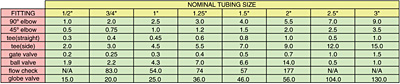
Start by getting the total equivalent length of the circuit. This consists of the length of pipe plus the equivalent lengths of other components, such as fittings and valves. Figure 2 lists the equivalent lengths of common fittings and valves.

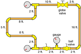
For example, the piping circuit in Figure 3 contains 62 feet of copper tubing within the flow path. It also has six 90-degree elbows, two “side port” tees, one straight-through tee, one globe valve and two ball valves. All tubing, fittings and valves are 3/4-inch size. The total equivalent length of this circuit is:

Le = 62 + 6x2 + 2x3 + 1x0.4 + 1x20 + 2x2.2 = 104.8 = 105 ft.

Once you have totaled up the equivalent length of the pipe, fittings and valves, use Formula 3 to determine the head loss curve.

Formula 3

Where:

k = value based on tube size from the table in Figure 4

Le= total equivalent length of circuit including tubing, fittings and valves (feet)

f = flow rate (US gpm)

1.75 = an exponent of the flow rate

Tube: k value

3/4-inch M copper: 0.00294

1-inch M copper: 0.000844

1 1/4-inch M copper: 0.000323

1 1/2-inch M copper: 0.000146

2-inch M copper: 0.0000396

2 1/2-inch M copper: 0.0000142

3-inch M copper: 0.0000061

3/8-inch PEX: 0.139

1/2-inch PEX: 0.0373

5/8-inch PEX: 0.0140

3/4-inch PEX: 0.00729

1-inch PEX: 0.00223

3/8-inch PEX-AL-PEX: 0.159

1/2-inch PEX-AL-PEX: 0.0393

5/8-inch PEX-AL-PEX: 0.00977

3/4-inch PEX-AL-PEX: 0.00333

1-inch PEX-AL-PEX: 0.00120

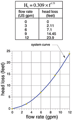
Here’s an example: We’ve already determined the total equivalent length of the piping circuits shown in Figure 2 (Le = 105 feet). The value of “k” for 3/4-inch copper tubing is found in Figure 4 (k = 0.00294). Therefore, the formula for the head loss curve is:

To make a graph of the head loss curve, just plug a few numbers for flow rates into this formula, calculate the head loss and plot the points. Finally, sketch a smooth curve through the dots to get the curve as shown in Figure 5.

Next month we’ll use this head loss curve to select an appropriate circulator. Stay tuned.