How to select a circulator using head loss and pump curves.

In the August issue, we looked at how to choose an appropriately sized pipe for a hydronic heating application. The procedure starts by estimating the flow rate needed to move heat to the load at a specified rate using an assumed temperature drop. Once the flow rate was estimated, the pipe size was selected based on keeping the flow velocity between 2- and 4-feet/second.

We also discussed the head loss of a piping circuit. You’ll recall that head is mechanical energy imparted to the fluid as it passes through the circulator, but dissipated from all other components the flow passes through. The faster the fluid moves through the circuit, the greater the head loss.

This month you’ll get the rest of the story. Specifically, how to select a circulator capable of producing the desired flow rate in a specific piping loop. The procedure uses both the head loss curve of the piping system and the pump curve of a “candidate circulator.”

Circulator Basics

The circulator is the heart of a hydronic circuit. It adds head energy to the fluid, creating the pressure differential that forces fluid to move through the piping circuit. An illustration of the cross section of a typical hydronic circulator is shown in Figure 1.

After flowing into the inlet port, fluid is channeled through the intake volute to the “eye” of the impeller. The eye is the hole through which fluid enters the impeller. Curved vanes on the spinning impeller then push the fluid outward between two disks. This is where head energy is transferred to the fluid. The fluid discharges from the perimeter of the impeller, and is gathered up by the outlet volute (the chamber in which the impeller spins). The fluid is then routed to the discharge port.

The flow rate of the fluid leaving the circulator is always the same as the flow rate entering the circulator. Assuming the inlet pipe and outlet pipes are the same size, the flow velocity entering the pump is also the same as the flow velocity leaving the circulator. However, the pressure of the exiting fluid is higher because of the added head. This increase in pressure is the “evidence” that head energy has been added to the fluid.

The ability of a circulator to move fluid cannot be expressed by a single number. Instead, it’s given as a graph called a pump curve. An example is shown in Figure 2.

Pump curves show how much head the circulator adds to the fluid as it flows through at a specific flow rate. For example, the circulator represented by the pump curve in Figure 2 adds approximately 12 feet of head to a fluid flowing through it at 8 gpm. A circulator always operates at some point along its pump curve.

To find the flow rate a given circulator will produce in a specific piping circuit, the system curve is drawn over the pump curve as shown in Figure 3.

The intersection of the curves is where the head supplied by the circulator exactly equals the head removed by fluid friction. This is called the “operating point.” The flow rate at the operating point is found by dropping straight down to the horizontal axis.

The flow rate produced by any given circulator may be greater than or less than the calculated “target” flow rate based on the rate of heat transport and an assumed circuit temperature drop. It’s purely coincidental if the flow rate at the operating point is exactly the same as the desired target flow rate. The goal is to select a circulator so the operating point is reasonably close to the calculated target flow rate. I would suggest an allowable variation of +/- 10 percent between the calculated target flow rate and that indicated by the operating point.

Using this method, the system curve of any piping circuit can be overlaid on the pump curve of any circulator to find what the flow rate would be if such a combination were to be used. The pump curves of several “candidate” circulators, all vying for the final selection, can be plotted along with the head loss curve for the piping circuit.

If you often select from a “palette” of say 10 circulator models on most jobs, you might want to make a graph showing all 10 pump curves. Then it’s just a matter of overlaying a given system to see what flow rate each of the circulators would produce in the piping circuit. Most circulator manufacturers now offer software that allows these comparisons to be made on a PC.

Flow Rates Without Flow Meters

The fact that a circulator always operates along its pump curve makes it possible to find the circuit’s flow rate without using a flow meter. All that’s required is an accurate measurement of the differential pressure increase across the circulator and a copy of the circulator’s pump curve.

The procedure requires the piping shown in Figure 4. This piping can be rigid and permanent, or flexible and removable. A single 0-30 psi pressure gauge is installed on a tee between two ball valves. Only one of these ball valves is open at a given time.

Using the same pressure gauge for both readings eliminates any absolute error in the gauge when one pressure is subtracted from the other.

Step 1

Open the ball valve on the inlet side of the pump and record the pressure gauge reading. Close this valve, then open the gauge on the discharge side and record the discharge pressure. Subtract the inlet pressure from the discharge pressure to get the differential pressure across the circulator.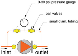

Step 2

Convert the differential pressure obtained in Step 1 to head gain using Formula 1.

Formula 1

H = ∆P(144/D)

where:

H added = head added to fluid by circulator

∆P = pressure increase measured across circulator (in psi)

D = density of the fluid (in lb./cubic ft.)

To use Formula 1 you’ll need the density of the fluid being pumped. This density should be based on the average temperature of the fluid in the circuit. A graph of the density of water at various temperatures is given in Figure 5. If using an antifreeze solution, look up its density in the manufacturer’s literature.

Step 3

Locate the head value calculated in Step 2 on the vertical axis of the pump curve graph, and draw a horizontal line from that value over to the pump curve. The intersection of this line and the pump curve is the operating point of the circulator. Draw a line straight down from the operating point and read the flow rate through the circulator on the horizontal axis.

Take The Test

Here’s a hypothetical design requirement for you to practice these calculations. You’ll need the data and methods for constructing a head loss curve given in the August 2003 column. If you don’t have this column, you can look it up in the editorial archives at www.PMmag.com.

Assume you need to design a piping circuit capable of transporting 100,000 Btu/hr. to a load using an assumed temperature drop of 20 degrees F. The circuit will use 200 feet of type M copper tubing. You’ve estimated the circuit will also contain forty 90-degree elbows, six straight-through tees and eight ball valves. The circuit will operate with water at an average temperature of 160 degrees F. Use the methods and data presented in this column and last month’s column to answer the following questions:

a. What flow rate is needed?

b. What diameter of type M copper tube should be used?

c. What flow rate will the circulator with the pump curve shown in Figure 2 produce in this circuit?

d. What is the head added by the circulator at this flow rate?

(Answers: a. 10.2 gpm; b. 1-inch copper tube; c. approximately 8.4 gpm; d. approximately 11.8 ft.)